Optimal control to expand

1.  Graph search optimal control in grid world as a starting point of the HJB equation, Chapter 7, underactuated robotics.
2. Dynamic programming from Kirk in discretized space using the previously stored state transition cost
3. HJB equation in continuous time optimal control, also linked to Dynamic programming. 
4. Assuming a solution/ S[N] expression for the HJB equation and then substituting it into HJB equation to see if it satisfies HJB and then getting the optimal gain from it.
5. Variational calculus approach to get the optimal control in continuous time from Naidu/Lewis
6. Dynamic programming based approach to get the Kalman gain matrix from Lewis for discrete system.
7. 
   

Things he did

1.  Made a finger gun and started shooting Phew Phew Phew for thre first time.
2. When asked to pour water, told to me that my mother asked him not to pour water.
3. Started singing Waka Waka song and dancing.
4. Complained to my mother that am taking sugar from his plate.
   

Journals for active magnetic bearing related work (AMB)

1. International Journal of Control, Automation and Systems, monthly, 55 days review, Link
2. Journal of Dynamical and Control Systems, once in 3 months, 5 days decisionLink
3. International Journal of Control, Automation and Systems, monthly, 55 days review, Link
4. IFAC Journal of Systems and Control, 2 weeks review,Link
5. International Journal of Dynamics and Control, once in 2 months, Link
6. Mechanisms and machine theory, monthly journal,3 weeks, Link
7. Mechanical systems and signal processing, monthly journal, Link
8. Sadhana,Once in 3 months, 40 days decision, Link
9. Journal of Vibration Engineering and Technologies, irregular publishing, First decisiton 5 days, Link
10. Journal of dynamics systems measurement and control, monthly journal, Link
11. Mechatronics, 3 months review, Link
12. Journal of Verification Validation and Uncertainity quantification, Once in 3 monthsLink
13. Archive of Mechanical engineering, once in 3 months, Link
14. The Journal of Vibration and Acoustics , once in 2 months, Link
15. International Journal of Systems, Control and Communications, once in 3 months, Link
16. International journal of control, automation and systems, open access, monthly journal,Link
17. European Journal of Control , 2 weeks publication, Link
18. Control engineering practice,once a year, Link
19. IEEE Transactions on Control Systems Technology , once in 2 months, paid Link
20. Frontiers in control engineering, 77 days review, Paid,Link
21. Journal of control science and engineering, paid, 31 days decision, Link

Paper Ideas to follow up

Current paper 2 plan (29 Oct 2022)

1. Show why 2D gain scheduling is required  +  2D gain scheduling considering speed and levitated height + LQR filter  for designing the PID controller in the gain scheduling + as you go lower, as you go closer to the bottom actuator, make the objective function take sign of the error into consideration, rather than simple xQx, quadratic under the effect of 1X disturbing force.

Notch filter based(29 Oct 2022)

1.  Instead of notching filter (Herzog 1996) + Tracking control for machining spindles, shift the notch filter central frequency around to balance between current consumption and vibration control. Also, based on the response to the 1X excitation force with the shifted notch filter, change the reference input adaptively: Called input trajectory optimization in https://ieeexplore.ieee.org/document/6859290, Nanu Chen

System identification + health monitoring (2 Nov 2022)

1. Do unbalance identification for health monitoring when the plant is originally controlled by LPV/gain scheduled control where RPM itself is a scheduling variable.

Active disturbance rejection control(29 Oct 2022)

ADRC is uses extended state observer ESO

ESO can be made time dependent, TADRC

Can you make ESO as parameter dependent (RPM ) dependent.

If ESO is itself state dependent (position) of plate, then does ESO become non linear. Can ADRC control it? "On disturbance rejection in magnetic levitation", Wei Wei, Wenchao Xue.

Algebraic successive integration scheme(29 Oct 2022)

1. FEM model with flexible rotor with algebraic successive integration for unabalance estimation and shaft model identification
2. Rigid rotor on AMB with algebraic successive integration for unbalance identification + km identification
3. Rigid rotor + AMB + algebraic successive integration for unbalance identification + Changing RPM + Notch filter tracking based on Herzog (03 Nov 2022)
4. Rigid rotor + AMB + algebraic successive integration for unbalance identification + Changing RPM + Notch filter tracking based on Herzog + With run out error on sensor disk (03 Nov 2022)
5. Impart thrust disk face out and thrust disk tilt on the 4 actuator supported thrust AMB, with rotation, in the first paper frame work on algebraic successive integration
   

 Also see older ideas:

https://balajimitplane.blogspot.com/2022/10/dyncont7-paper-publication-ideas-to.html

DynCont#10 Linearising closed loop in simulink, Equilibrium point, trim point.

1.  When linearising a non linear plant, about a trim point, always open the feed back loop
2. Do not place input perturbation and output pickup in simulink in the closed loop
3. Linearising is applicable for unstable systems, so open the feedback loop and linearise the plant alone.
4. Important : Trim point is not Equilibrium point
5. At equilibrium point, all state vector derivatives are zero
6. At trim point, only the constrained state vector derivatives are zero. Example, linearising the aircraft model at a constant forward speed.. 

 

From Analyzing Models (Getting Started) (urv.es)

DGI direct gasoline injection system drive details

1. Purchase link: GDI_CRDI_Direct_Injector_Tester (autodiagnosticsandpublishing.com)
2.  Good article on current sense and drive circuit : Link
3. NCS 333 Operational amplifier.. Link
4. BSS123 Mosfet: Link
5. Using pressurised nitrogen bottle and to pressurise the fuel line instead of using a DGI pump: Mdpi paper on bike engines DGI optimisation.
6. A good reference with details on the circuit design of the DGI injector drive circuit and the power stage: 2011 Paper (Wenchang Sai)
7. High pressure DGI injector drive circuit using 3 Mosfets : 

   

   High pressure 3 stage pulses injector drive circuit PCB from MDPI paper

   
   
8. Study of the injector drive circuit for a high pressure GDI injector, Simulation study: Link
9. Some photos of the experimental setup in Professor Krishna Sahu's Lab, thermodynamics:

10. 

    Ford injector 

    
    

    

    Fuel rail with the injector

    
    

    

    Cam driven DGI pump

    
    

    

    Encoder for triggering the solenoid of the cam driven DGI pump

    
    

Specifying design point of a gas turbine: Lesson learnt.

1. Design point of the compressor for a gas turbine is specified at 100% RPM, 101325 Pascal inlet pressure and 288.15 at  0 Mach = ISA SLS
2. Design point performance of the compressor is specified as 3 numbers
1. Corrected mass flow rate
2. pressure ratio
3. efficiency
3. The inlet face of the compressor is at ISA SLS
4. If you have inlet pressure drop in the bell mouth inlet at ISA SLS, then actual mass flow rate seen by the compressor will be less than the corrected mass flow rate. 
5. For design point calculation, do not give inlet pressure drop in the bell mouth inlet.
6. If inlet pressure drop in the bell mouth inlet is zero, the actual mass flow rate and corrected mass flow rate will be same and it is easier to generate the compressor characteristics curve from CFD.  
7. Commercial softwares such as GSP change the design point Mach number automatically when you specify the inlet pressure drop. For example, if you give design point ISA SLS inlet pressure drop as 0.98, it will automatically raise Mach number to 0.17 and reduce the ambient temperature by 2 degrees. 
8. The raise in total pressure at the inlet due to Mach number compensates for the inlet pressure drop and the compressor corrected mass flow rate and actual mass flow rate are same. inlet face of compressor sees 101325 after the total pressure rise due to mach number and total pressure drop due to inlet pressure loss.
9. The reduction of ambient temperature by -2 degrees compensates for ram temperature rise and compressor inlet temperature  becomes 288.15 after Mach number total temperature rise 
10. If you want zero mach number with inlet pressure drop, use the "flight" option in GSP and not the design point calculation option. 

DynCont#9 Simple Looped AI and AO using PXIe, nidaqmx, Python, Labview, NIMAX

1. It took 3 days of poking, trial and error to get this python program working. This can only be run with hardware (PXIe system, with NI 6356 card. It has 8 diff analog inputs and 2 analog outputs
2. No, you cannot use 8 differential as 16 ground referenced single ended channels. Pay more for that to Hungary.
   
3.  LABVIEW not essential
4. NIMAX drivers required for configuring connections, checking hardware using test panels
5. nidaqmx python library used instead of labview.
6. LABVIEW is a mind melting mixed veg noodles, that is 2 days old.
7. This program is a simple looped AI and AO 
8. It is not yet software timed. To do software timed loop, use a while loop inside the outer loop to check if your control loop update time has elapsed and then continue with the next outer loop pass.
9. In software timed loop, if one outer loop pass takes more time than your control update time, then increase control update time.
10. In hardware timed loop, use call backs from input task that is triggered after samples are read from the buffer to the computer.
    
11. Program below samples  4 channels of analog in TCV, BCV, Excitation and Eddy. Writes 2 outputs TCV and BCV. TCV and BCV are looped into analog in also.
12. No hardware or software timing, no processing using the sampled values to calculate the outputs. Only seeing how fast simple loop runs. This is the bare minimum control update possible. This uses stream readers and stream writers. Uses shared clock between analog in and analog out. Uses a trigger from analog in to start analog out.
    

DynCont#8 NIDAMX PID control Labview NI PXI

Tasks start and stop behavior:

1.  If you are using finite samples, no need to stop after reading input. Always close only at the end of the complete program
2. Create task once in the beginning of the program
3. Start task once when using finite samples.
4. If you allow regeneration, call backs will not work: Source = https://forums.ni.com/t5/Multifunction-DAQ/Continuous-write-analog-voltage-NI-cDAQ-9178-with-callbacks/td-p/4036271/page/2?profile.language=en

Don't use  USB/ETHERNET

If you are using a USB DAQ, keep in mind that the devices are optimised for data throughput not response latency. You don't want to service tasks (e.g. pull data off the board) more than about 5 times a second. Consequently you should plan to perform larger operations on a USB DAQ than on a PCI or PCIe-based device.

Source: https://github.com/tenss/Python_DAQmx_examples

Software timed IO:

Source = https://www.ni.com/docs/en-US/bundle/ni-daqmx/page/mxcncpts/controlappcase5_2.html

1. For software timing, the software and operating system determines the rate at which the loop executes. Software timing is not deterministic. Controlling a while loop and using the Wait Until Next ms Multiple VI to handle timing is an example of a software-timed loop. 
   
2. IO is triggered by the python code in the PC
3. Use this mode when hardware time IO is not available
4. Timing will have jitter due to software errors
5. Configure the Timed Loop to run at the desired rate. 
   

Hardware timed IO:

source = https://www.ni.com/docs/en-US/bundle/ni-daqmx/page/mxcncpts/controlappcase1.html

1. The current iteration's output samples are guaranteed to be aligned with the next iteration's input samples. 
2. Use the DAQmx Wait For Next Sample Clock function
3. Read, process, and write operations are confined to the time available between the moment the device starts acquiring data and the moment the next sample clock edge arrives.  
4. Does exactly what we need = An example of this kind of application is an analog control loop that reads samples from a specific number of analog input channels, processes the data using a control algorithm (such as PID), and writes new control values to the analog output channels.  

Software develop helps

1. https://github.com/mjablons1/twingo
2. https://github.com/toastytato/DAQ_Interface
3. https://github.com/czimm79/MuControl-release
4. Relevant = https://github.com/tenss/Python_DAQmx_examples
5. Relevant = https://github.com/mjablons1/nidaqmx-continuous-analog-io
6. Relevant = https://github.com/mjablons1/nidaqmx-continuous-analog-io 
   
7. https://github.com/tenss/SimplePyScanner
8. https://github.com/petebachant/daqmx
   
9. https://github.com/tenss/Python_DAQmx_examples/blob/master/pynidaqmxegs/mixed/AOandAI_sharedClock.py
   

DynCont#7 Paper publication Ideas to follow up.

 Controls

1. PD control steady stater error in servo control analysis and physical meaning
2. PD / PID + Mapping of the initial trajectory required + Using preknown offset to modify the desired path beforehand from system identification +  Tune this controller using LQR using closed form algebraic solution of Ricatti equation 
3. Weight the negative error more than the positive error to simulate the non allowable tool plunging while optimizing LQR (x^3-x^2-x)^2 rather than x'Qx. 
4. Model reference adaptive controller . 
5. Mode predictive controller for AMB 
6. RAMB. Flexible mode control using RAMB. How to damp the flexible modes.
7. Simulation model of shaft on AMB with Dynamic modal decomp, sparse SINDY, DMD with control , DMD without control!...
8. Kalman filter post on linked in https://bitbucket.org/tremaineconsultinggroup/observer_luenberger/src/master/
   

 Gas turbines

1. PID controller with gain scheduling for gas turbine
2. LQR / LQG controller for gas turbine
3. MPC controller for gas turbine
4. Model reference adaptive controller for gas turbine

Foil bearings

1.  Link model FEM from IISC course+ Psedospectral method
2. Orbit simulation
3. Stability analysis
   
4. FDM  / FVM / Commercial solver comparison for Foil bearing
5. Software for foil beairng load capacity estimation

DynCont#6 Optimal control resources for preparation

• Video lectures =  AA4CC lectures (Lecture 2 missing)
• Video lectures = Neuro match academy, good explanation, https://www.youtube.com/playlist?list=PLkBQOLLbi18NSMbvuDS2WaXLWctg3QArY
• Video lectures = Barjeev Tyagi, IIT Roorkee, https://nptel.ac.in/courses/108107098
• Video lectures - Shyam Kamal, IIT BHU, EE564,  https://www.youtube.com/playlist?list=PLHEIL5MR2cEGqWdrFvzxDwR6Lw-D5ETWY
• Video lectures = G D Ray, IIT KGDP, https://www.youtube.com/playlist?list=PLbMVogVj5nJQNzJT6sYZpB7H1G6WF0FZ4
  
• Optimal control 2022 https://www.youtube.com/playlist?list=PLZnJoM76RM6Iaf59ICcU9-DzztGZvK_52
  
• Kirk Introduction to optimal control book
  

Investing in India - Points from Nitin Kamat, Zerodha

Trade volume

1.  90% of the trades made in Indian stock market is done by traders doing intraday. They are 3% of the DEMAT account holders
2. 97% of people are doing investing and not intra day
3. This 97% of people contribute insignificantly to the trade volume in India

Growth expectation by Venture capitalists

1. VC investors want growth. Not profitabilityFor VC, it is ok to spend 400 Rs for customer acquisition who will give 200Rs profit at the max
2. VC will have 7 year investment cycle
3. VC 1 will have to exit after 7 years, selling the share to another VC, who will have sell to another .
4. For first VC to exit and second VC to enter, there should be growth in the company.
5. If there is good growth and good potential for future growth, why will first VC exit after 7 years?
6. Where will he invest after exiting?
7. VC1 has to invest in another startup after exiting. Why not stay with the company where he has understood the business and know the founders for 7 years? 
8. If VC 1 is convincing the next VC that growth is going to be there, why VC1 is exiting ?

 

 Growth expectation by market

1. It is not enough for a company to make profit or stay sustaibable
2. Company has to keep growing. A company that does not grow will be de-valued even if it is sustaibable and is profit making. Example = Coin base
3. India , 140 crore people have less than 2 Lakhs per year.
4. They will not invest in stock market, even if brokerage is free.
5. Growth base for fintech companies is not the population, it is the IT paying population, less than 1% of the population.
   

Matlab program to plot the magnetic bearing constant and force values from the E actuator

Second set of experiments on April 25,2022 with old load cell plotting.

Third set of experiments on August 29,2022 with new load cell plotting

FEMM program in Matlab to obtain the forces from EI core electromagnetic actuator for different gaps and current.

 The top surface of the E actuator, facing the thrust plate is not flat due to previously unknown error in the surface grinder bed level.

The top of the E actuator needed to be all at 40mm, but they were differing to a max of 140 microns above the mean as shown below. When the thrust plate was touching the top surface of the E actuator, it was actually 140 microns above the center leg, not flush with the actuator. The forces that were measured with the load cell are actually at a higher gap than the gap measured with the eddy current probe.

The uneven top surface due to error in surface grinding operation

PID control resources for NI system

 LABVIEW Vi for implementing a single channel PID controller: 

https://knowledge.ni.com/KnowledgeArticleDetails?id=kA00Z0000019QlFSAU&l=en-IN

Use queue and channel wires

Use QUEUE to communicate between analog read and analog write task

 

One portion of code is creating (or producing) data to be processed (or consumed) by another portion. The advantage of using a queue is that the producer and consumer will run as parallel processes and their rates do not have to be identical. 

 

https://knowledge.ni.com/KnowledgeArticleDetails?id=kA00Z000000P7OfSAK&l=en-IN 

https://www.ni.com/en-in/support/documentation/supplemental/16/channel-wires.html

PID control labview example video:

https://www.youtube.com/watch?v=lyw_Ygeti3I&ab_channel=NIDevZone

https://www.youtube.com/watch?v=qMydcfZ_ZSs&ab_channel=FlexRIO

Thesis on PID control with labview

 

http://www.diva-portal.org/smash/get/diva2:757138/FULLTEXT02

https://www.ni.com/en-in/innovations/white-papers/06/pid-theory-explained.html

 

Simple on off control LABVIEW

Source

Basic on off control using labview

 

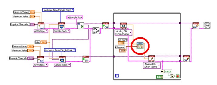Hardware timed PID control using shared sample clock and trigger

PID control with python and NIDAQMX

https://halvorsen.blog/documents/programming/python/resources/powerpoints/Control%20System%20with%20Python%20-%20Air%20Heater%20System%20-%20Part2.pdf

 

Edit on 15 Oct 2022

From https://forums.ni.com/t5/Multifunction-DAQ/Continuous-write-analog-voltage-NI-cDAQ-9178-with-callbacks/td-p/4036271?profile.language=en

 

1) Your code comments refer to wanting to be able to update output signals at 100 Hz, presumably under software control.  I assume this means you want <= 10 msec latency between your software deciding on an output value and having that output appear as a real world signal.     This is pretty tricky to accomplish with a buffered output task, and (I suspect) likely impossible when the device is connected by USB or Ethernet.  You may need to approach this with an unbuffered, software-timed, "on-demand" task and then live with the corresponding irregularities and uncertainties of software timing

2) The rule of thumb wouldn't apply to situations where low latency is the priority.  A lot of typical data acq and signal generation apps don't need real-time low latency.  They generate pre-defined stimulus signals and collect data for post-processing later.  The rule of thumb works well in those cases, allowing live displays with only *moderate* latency, enough for an operator to see what's going on.

3) In the past when I experimented with trying to do low latency hw-clocked AO, it wasn't trivial to get < 10 msec even with a PCIe device.  I recall that in order to get there, I needed to set up a few different low-level and fairly advanced DAQmx properties to non-default values.  I wouldn't have expected the defaults for a cDAQ system over USB to support that kind of usage so easily.

4) 

Sample rate and samples per channel

 

Sample rate is how fast you sample a signal.  Samples per channel is the size of buffer alloted per channel.  If you have a sample rate of 1000 samples/s, and you have 1000 sampels per channels, your buffer will overflow if it is not read before 1s elapsed.  you always want to set your samples per channels a few times over your sampling rate

 

Hardware timed single point

Link = For deterministic timing, do not use CDAQ. Only in CRIO or PXI 

Time stamping of acquired data samples from NI DAQ devices.

1. DAQ cards do not have a time stamp mechanism, so we use the t0 (Buffer read time, not task start time) and dt in LabVIEW to time stamp it. Link = https://forums.ni.com/t5/Multifunction-DAQ/Loop-timing-with-NIDAQmx-for-Python/td-p/3656140
2. DAQmx does not timestamp samples when they are taken on the DAQ device, but it does when it reads the FIFO samples onto the computer if you are reading in a waveform data type.
3. Read = Reading from the FIFO buffer  into the PC
4. Acquire = Acquisition of data by the DAQ hardware
5. SOlution =  Each time you acquire, note down the time when the specific loop interation starts and then append dt to it for every column.
6. Every row is a channel
7. Every column is a sample taken in that channel.
    

Program for design point cycle analysis and parametric analysis of turboprop engines and plotting of parametric results, gas path temperatures and pressures.

Python program for controlling NI-cDAQ device without LABView installation

1.  Requires NI-MAX driver more than 17.0
2. Lots of dependencies for nidaqmx python wrapper for the C API given by NI
3. Plotting is using Matplotlib
4. Use pip download option to download all the required dependencies as whl files on the computer with internet and then transfer the folder with whl files to the DAQ computer that is without internet
5. Use pip install --find-links --no-index option to install the nidaqmx on the DAQ computer without internet
6. The python program below generates signals used to excite the power amplifiers.Force from power amplifiers is measured via FX293 load cells via NI9205 input card.
7. Generation and acquisition tasks must be committed before being used. Other wise there is big lag between start of generation task and start of acquisition tas
8. See if you can use same clock source for both generation and acquisition to ensure synchronous use
9. Trigger can be used on output task. Output tasks trigger is given by input task. input task should be committed before taking trigger from it.
10. If you are using a task in a loop, always close the task for each loop use. Other wise the task will not read new data.
11. Program below:
    

NIKOTTO presentation on IC engine DAQ

• NIKotto  = startup by IITM PHD students
• Data acquisition through NI PXI system 
• Data transferred from NI PXI to workstation through LAN
• Python code does data processing in workstation
• DASH python used for making UI running in browser connected to local host
• Data is stored in file formal HDF5
• DASH good for presenting plots, writing reports
• 
   

STM 32 programming

https://www.youtube.com/watch?v=VlCYI2U-qyM&ab_channel=Phil%E2%80%99sLab

 

 STM32 can be programmed via

1. Not clear: Serial wire debug = SWD
2. Not clear: JTAG
3. DFU= Device firware upgrade 
1. ( No provision of setting break points in DFU mode)
2. Use application note AN3156 
3. STM32 Cube programmer software use elf file as input
4. STM32 Cube programmer can upload using 
1. STLINK
2. USB
3. UART
5. Boot zero pin to be pulled to high and restart the MCU to put the MCU in the DFU mode.
6. After flashing the elf file to the MCU using the STM32 Cube programmer, pull boot 0 pin low, restart the MCU
   
4. Not clear: Via USB = You have to write your own boot loader for this.
   

DynCont#5 Fixed and relative frames of reference in high speed shafts

1.  We always measure the speed only in the fixed frame of reference, inertial, non accelerating, constant velocity.
2. It is easier to do integration in ground fixed, inertial frame of reference.
3. But for a whirling shaft / tumbling body, the mass moment of inertia along the x axis of fixed frame of reference keeps changing due to the tumbling of the disk,even though the disk is rigid.
4. For an axis system that is aligned to the disk at a particular instant in time, not fixed to the disk, the mass moment of inertia along the x axis of the aligned system is constant.
5. But it is difficult to do time integrations along this axis system that is aligned to the disk 
6. Again, we are only measuring with respect to ground fixed reference system. That value, we are expressing in terms of an axis system that is aligned to the disk at that particular instant of time. This is only to use the inertia defined in the disk aligned axis system. With this kinetic energy, we can write the Lagrange governing equation and then derive the fundamental equation of motion. 
   

Skills

Mathematical modeling

1.  Development of physics based models for mechanical systems from fundamental equations.
2. Development of plant models using system identification techniques from test data with various control inputs (Step, impulse, sine sweep, PRBS)
3. Development of performance augmentation controllers / Stabilising controllers using
1. PD
2. PI
3. PID
4. LQR
5. State space control
4. Development of simulation models in 
1. Python using numpy/scipy
2. Matlab with Simulink.
5. Tuning of controllers using the simulation models

Embedded programming /  Electrical schematics / PCB

1. Implementation of control algorithms in C for TI MCU / AVR MCU / C2000 DSP
   
2. Design of electrical schematics for controllers and power circuits
3. Design of signal conditioners for ADC and DAC
4. Simulation of electrical schematics using LTspice/Falstad
   
5. Design of PCB (low speed upto 5kHz) 

 Mechanical design

1. Design of test rigs using Solidworks : Dimensioning/TOleranceing GD &T as per ASME standards
2. Optimising design for assembly and manufacturability.
   
3. Design of sheet metal structures for equipment , test rigs and protective enclosures.
4. Design of welded structures / frames
5. Follow up : Fabrication of machined parts : CNC turning center / VMC machining center.
   
6. Follow up :  3D printing (ABS/PLA/PCA)
   

DynCont#5: Z transform, Phils Lab, DDorran

Phisl lab

1.  Z transform is better than Fourier transform because it can do 2 things:
1. Check the stability of the implemented difference equation
2. See the frequency response of the system, that the difference equation represents
2. Z transform based stability check: Simple, replace y[n-1] by z^-1 Y and form the Z transfer function and check the location of poles . Zeros can be out side the unit circle for stable system
3. Z transform based frequency response z^(-k) = e^(-j theta k), where theta  = 2*pi*f/fs. Maximum value f can take is fs/2 so maximum value theta can take is theta = pi. 
4. For DC gain, omega is zero so z = 1
5. For high frequency gain, z= -1

 DDorran

1. Z transform is used to detect the presence of exponentially increasing or decreasing components in the signal
2. By identifying the increasing or decreasing oscillations in the impulse response  of a system we can determine if that system is stable or unstable
3. x[n] is a signal with different values for different n. z^(-n) is also a signal for different values of z. Multiplying individual values of the 2 signals and adding them is basically taking correlation of 2 signals. Higher the correlation, more is one signal present in another signal
4. Correlation is the measure of presence of one signal in another signal.
   
5. When taking correlation of 2 signals, note that if second signal is constructed using z = 1, then we are basically taking the DC value of the first signal. Also see 4th point of previous stack.
6. Z is e^(-sT). Value of the z transform at z = 1 in the plot with z values as x axis is the DC value of the signal.
    

New things he did.

1.  Started saying 2 word sentences in the second week of July 2022
2.  Started saying 3 word sentences in the second week of July 2022, like "Mukesha Amma kupudranga!" to Mukesh who was playing inside.
3. Went to Priya office for full day without going to school so that me and mother can go to Vaniyambadi for Manju funeral. Next day, he asked mother to go to shop and me to go to office so that he and Priya will be alone in the morning and she will take him to office in Bus rather than go to school.
4. Started saying all options other than school. "Priya, Bus train auto polama?"
5. Started identifying a train when we cross a train track near BEML gate and started asking shall we go in train whenever we cross BEML gate.
6. Started adding his own words into conversations : When Priya told me to buy chocolate and cake from behind on the bike, I asked her to repeat as I could not hear what she told. Him, sitting, inbetween told, "Chocolate, ice cream, cake". 
7. When we go to drop Priya in the morning, he starts crying that he wants to take his bag too. So that he can take his bag and go to Priya office rather than school.
   

Notes Random

1. Best drill bits to buy, even if you are drilling rocks: PDC = poly crystaline diamond compacts
2. Why Tungsten Carbide drill bits are better than HSS drill bits?
1. Tungsten carbide drill bits have to be sharpened only by diamond wheels, so their sharpening is done on good machines whose angles are controlled precisely. So they make better drill bits
2. HSS drill bits are cut in normal grinding wheels, so their angles may not be as precise and process may not be strictly controlled. This results in poorer drill bits in the end
   
3. Both Cobalt and Nickel are used as binder in Tungsten Carbide drill bits. When nickel is used, the bit is slightly magnetic. When cobalt is used ?
   
4. Cobalt has higher thermal expansion and so when Cobalt binded Tungsten Carbide drill bits are used for long, due to thermal expansion, they may fail.
5. Always have UV seals next to the commutator brushes in the motor. Constant sparking of the commutator brushes give out UV light and the light damages the polymer cage of the bearing and the grease.
   

 

DynCont#4: SVD, 3Blue1Brown

1.  If determinant is zero, the transformation matrix collapses the input vector to a point in the output vector space
2. A span of the vector is a line , infinite passing through the vector in both the directions. A vector can be multiplied by a constant number and the head of the vector will be somewhere along the line for different constants 
3. Matrix multiplication:
1. Row wise picture, conventional computational approach
2. Column wise picture
3. Transformation from one vector space to another vector space approach
4. Will be edited after listening to the lec again.
   

Notes, random

1.  No point in anticipating and worrying.
2. Know the scenario as best as possible and then start worrying about it so that you can worry effectively.
3. If some one is coming to you, he wants something from you. It may be knowledge, but consider how that knowledge will be used.
4. Some people may not have points of contacts at all. Not interested in talking to you or getting information from you. Not all people are same.
5. Survival is not every thing?
   

Cosmic view points: Purpose of universe

1. The egg, short story by Andy Weir : Purpose of universe is to mature us.
   
2.  Actions of intelligent life are an unfortunate irrelevance in the majestic universe of stars and galaxies. It is bad manners to  give too much importance to intelligence/Love= Emotion
   
3.  Only purpose of universe is to produce intelligent sentient beings. Other astronomical phenomena is just dead matter.

 

 

DynCont#3: SVD, MIT 18.065 Strang you tube lecture video 6

1.  We are looking for a bunch of orthogonal vectors u, which when multiplied by A, give another set of orthogonal vectors v, scaled by sigma
2. Curse of Dimensionality =   A matrix is basically scaling and rotation. For a 2x2 matrix, there are 4 terms . it has 2 scaling values and 2 rotations. The rotations increase the time taken. not the scaling. For 3x3 matrix, there are 9 independent terms with 6 rotations and 3 scaling terms. Similarly, 4x4 matrix has 4 scaling terms and 12 rotations.
3. Rank= If A has rank r, there are r orthogonal vectors , which when multiplied by A give another r orthogonal vectors.
4. If U vectors are orthogonal in AU=sigma V, it can be proven that V vectors are orthogonal by simply substituting VV' = (AU/Sigma1)* (AU/Sigma1)'

DynCont#2: SVD, MIT 18.065 Strang you tube lecture video

1.  A * v = u * Sigma
2. Matrix A times an orthogonal vector matrix = another orthogonal vector matrix scaled by sigma
3. Sigma is diagonal matrix
4. Sigma is the square of eigen values of A A'
5. AA' is symmetric and positive semi definite 
6. If A is mxn, AA' = m x m . Then, it will have m eigen values.
7. If A is mxn, A'A = n x n . Then, it will have n eigen values. If m is greater than n, then m-n eigen values of AA' will be zero.
8. Use of SVD:?
9. SVD from lecture 29 in 18:06?
10. Use of SVD from Knuth?
    

 

DynCont#1: SVD, Knuth you tube lecture video

1.  Singular value decomposition exists for all rectangular matrices
2. A square is a rectangle
3. LR , LQR, LU may not exist for some matrices
4. All matrices are basically rotation and stretching.
5. A = ULV'
6. U and V are rotations
7. L is the scaling 
8. L square will have the eigen values of AA'
9. U and V are orthonormal matrices, so their inverse and transpose are same
   
10. 
    

Hacker earth C programming question and answer

 Problem

You are given a table with rows and columns. Each cell is colored with white or black. Considering the shapes created by black cells, what is the maximum border of these shapes? Border of a shape means the maximum number of consecutive black cells in any row or column without any white cell in between.

A shape is a set of connected cells. Two cells are connected if they share an edge. Note that no shape has a hole in it.

Input format

• The first line contains 

lines contains

• integers.

Output format

Print the maximum border of the shapes.

Sample Input

10
2 15
.....####......
.....#.........
7 9
...###...
...###...
..#......
.####....
..#......
...#####.
.........
18 11
.#########.
########...
.........#.
####.......
.....#####.
.....##....
....#####..
.....####..
..###......
......#....
....#####..
...####....
##.........
#####......
....#####..
....##.....
.#######...
.#.........
1 15
.....######....
5 11
..#####....
.#######...
......#....
....#####..
...#####...
8 13
.....######..
......##.....
########.....
...#.........
.............
#######......
..######.....
####.........
7 5
.....
..##.
###..
..##.
.....
..#..
.#...
14 2
..
#.
..
#.
..
#.
..
..
#.
..
..
..
#.
..
7 15
.###########...
##############.
...####........
...##########..
.......#.......
.....#########.
.#######.......
12 6
#####.
###...
#.....
##....
###...
......
.##...
..##..
...#..
..#...
#####.
####..

 denoting the number of test cases.

The first line of each test case contains integers 

 denoting the number of rows and columns of the matrix. Here, '#' represents a black cell and '.' represents a white cell. 

Each of the next 

My solution

#include <stdio.h>

#include <stdbool.h>

int main(){

    int numDataSets,numRows,numCols,maxPatternSize;

    bool patternStarted = false;

    

    // Dynamic heap arrays

    char *rowDataPtr;

    int *rowWisePatternLengthsPtr;

    int *dataSetWisePatternLengthsPtr;

    scanf("%d", &numDataSets);      // Reading number of data sets

    //printf("Number of data sets is %d.\n", numDataSets);

    // Create an integer array to print all the row wise pattern lengths at the end

    dataSetWisePatternLengthsPtr = (int*) malloc (numDataSets * sizeof(int));

        

    for (int i=0;i<numDataSets;i++)

    {

        //printf("\n==========================================");

        //printf("\nData set = %d",i);

        // Get number of rows and cols in each data set

        scanf("%d", &numRows    );     

        //printf("\nNumber of rows in this data set %d is %d",i, numRows);

        scanf("%d", &numCols    );     

        //printf("\nNumber of Cols in this data set %d is %d",i, numCols);

        // Create an integer array to print all the row wise pattern lengths at the end

        rowWisePatternLengthsPtr = (int*) malloc (numRows * sizeof(int));

        

        //Take in one row of the data at a time.

        for (int rowNum=0;rowNum<numRows;rowNum++)

        {

            //printf("\n Row number = %d : ", rowNum    );

            patternStarted = false;

            rowWisePatternLengthsPtr[rowNum] = 0;

            // In each row, assume that the pattern has not started and pattern length is 0

            // Create a char array dynamically on the heap

            

            // Adding 1 so that new line can be stored?

            rowDataPtr = (char*) malloc ((numCols+1)*sizeof(char));

            if (rowDataPtr == NULL)

            {

                printf("\n Could not allocate the memory for row %d",rowNum);

                printf("\n Required column size = %d",numCols);

            }

            // Scan all characters of the row

            for (int colNum=0;colNum<=numCols;colNum++)

            {

                scanf("%c", &rowDataPtr[colNum] );     

                //printf("\n Column number %d is %c", colNum,rowDataPtr[colNum] );

            }

            // Print all characters of the row for checking

            for (int colNum=0;colNum<=numCols;colNum++)

            {

                //printf("%c", rowDataPtr[colNum]   );     

            }

            for (int colNum=0;colNum<=numCols;colNum++)

            {

                if ((rowDataPtr[colNum] == '#') && (colNum != numCols))

                {

                    patternStarted = true;

                    rowWisePatternLengthsPtr[rowNum]++;

                }

                if ((rowDataPtr[colNum] == '.') && (patternStarted == true))

                {

                    patternStarted = false;

                    break;

                }

            }

            //printf("Row wise length = %d\n",rowWisePatternLengthsPtr[rowNum]);

        }

        // Find the maximum number of stars in the array rowWisePatternLengthsPtr for this data set

        maxPatternSize = 0;

        for (int rowNum=0;rowNum<numRows;rowNum++)

        {

            if (rowWisePatternLengthsPtr[rowNum] > maxPatternSize)

            {

                maxPatternSize = rowWisePatternLengthsPtr[rowNum];

            }

        }

        dataSetWisePatternLengthsPtr[i]=maxPatternSize;

    }

    for (int i=0;i<numDataSets;i++)

    {

        //printf("\ndata set num %d= %d",i,dataSetWisePatternLengthsPtr[i]);

        printf("\n%d",dataSetWisePatternLengthsPtr[i]);

    }

}

Literature survey for RTA class aircraft engine

 

Rolls Royce DART

Figure 1 Rolls Royce DART turboprop

 

Rolls Royce Dart is a pioneering turboprop originally designed in 1945 that is still in service today. It is simple single shaft turboprop with a 2 stage compressor with both the centrifugal stages being the superchargers of Eagle and Griffon piston engine. A single 2 stage turbine drives both the compressors and the propeller. The later variants have 3 stage turbines. The production was continued till 1987. Dart 21(1910 SHP) has a mass flow rate of 9.7 kg/s and the much later Dart 201 (2970 SHP) has a mass flow rate of 12.25 kg/s.

The intake to the engine is a circular one with an annular duct leading to the eye of the first stage centrifugal compressor. Oil tank around the intake is cast integral with the casing of the compressor. A secondary air intake supplies air to the oil cooler mounted on top of the centrifugal compressor casing. The centrifugal compressor is in tandem arrangement on the same shaft. Each impeller has 19 vanes and has guide vanes made from steel. The combustion chamber is a straight flow combustion chamber. The tubes are arranged diagonally to increase the burning length. The flame tube has fuel atomizers at the front end of each tube for downstream injection. The igniter plugs are placed in number 3 and number 7 chambers of the combustor. The turbine is an axial flow type and has three stages. All blades are of made from Nimonic alloy and are secured on the disk by FIR tree roots. The jet pipe is coaxial with the engine main shaft, but the exhaust unit has a slight inclination to suit the installation on the aircraft. Maximum temperature in the jet pipe is of the order of 650 degree Celsius. The output from the engine is through a double reduction gearbox with helical high speed gear train and a final helical gear drive. The two gear trains are connected by three lay shafts to distribute the torque from the driving gear to the driven gear. All gears and propeller shaft are carried in roller or ball bearings. Bevel gears from one of the lay shafts provide the necessary drive for the fuel pump, oil pump and the propeller control unit.

 

Rolls Royce Tyne RB 109

Figure 2 Rolls Royce Tyne turboprop

         

Rolls Royce Tyne Is a twin spool turbo prop that set new high standard for the pressure ratio and fuel economy when it was designed in 1955. The engine is very successful and was in production for 30 years with the last engines delivered in 1990s. The Tyne -22 engines powered the Transalls C-160 aircraft in Germany until 2019. Safran aircraft engines, under contract with the French Government, is committed to provide Tyne 21 to the French Navy up to 2035.

          The Rolls Royce Tyne has an annular intake that is similar to the AI20 series with seven hollow supporting struts. This annular intake surrounds the reduction gear box housing and is cast in magnesium alloy. This casing also forms part of the oil tank which is also annular. Anti-icing is done by hot oil circulated through the hollow struts and by hot air tapped from the high pressure compressor .

          The low pressure compressor has six axial stages whose rotor discs are made of steel. The first stage rotor disk is integral to the shaft. The other 5 stages are splined to the shaft. The rotor blades are made of “216 light alloy” and are fixed to the rotor disk with individual steel pins. The stator blades are made of “431 aluminium alloy” and fixed using tongues in groves. The first stage stator blades are hollow and use HP bleed air for anti icing. First stage also has provisions for water injection to increase power in take off rating. Both the front and rear bearings are roller bearing type. The entire low pressure section casing is a single piece steel unit. Bleed valves are used in the top casing to prevent surge whenever LP and HP spool speeds are unmatched.

          The high pressure compressor has 9 axial stages made of steel discs. The first 2 stages are attached to the shaft with steel bolts. The other 7 stages are fit using splines on the shaft. The rotor blades of the first 7 stages are made of Titanium and the last 2 stages are made of steel. The HP stator blades are made of “734 steel” and the casing is also a centrifugally cast steel component. The front bearing is a roller bearing while the rear bearing is a ball bearing. The pressure ratio and mass flow are similar to AI20, being 13.97:1 and 21.1 kg respectively.

          The combustion chamber is a 10 flame tube can-annular type. The tube are made of Nimonic steel and the annular casing is made from sheet steel. The flame tubes contain double twin-flow coaxial burners. The high energy igniters are in tubes 3 and 8.

          The high pressure turbine is made of single steel disk with Nimonic blades attached to it using FIR tree roots. The steel disk is bolted to the shaft using 10 tapered bolts. The high pressure turbine shaft is splined on to the high pressure compressor shaft. The rotor blades are tip shrouded. The stator vanes and rotor blades are air cooled. The casing is centrifugally cast steel. The gas temperature is of the order of 1000 degree Celsius.

          The low pressure turbine has 3 stages. The low pressure turbine shaft is splined on to the low pressure compressor shaft. The last rotor of the stage 3 is integral to the shaft. All the rotor blades are made of Nimonic alloy and are attached to the disks using FIR tree roots. The first stage LP nozzle guide vanes have thermocouples at their leading edges. The temperature at the exit of the LP turbine is 453 degree Celsius. The read of the low pressure turbine shaft is supported on roller bearings and the front of the shaft rides on the high pressure turbine shaft on a plain bearings.

          The epicyclic gear train is driven from the front end of the low pressure compressor shaft. The planet wheel carrier of the final drive is integral to the propeller shaft. The gear ratio is 0.064:1. Various propellers ranging from 4.42m diameter to 5.49 m diameter are used with this engine. The gear box also incorporates a torque meter. The entire engine weighs around 995 kg (Mk 515) and produces 5730 equivalent HP (Mk 515).

 

 

Allison / Rolls Royce 501

Figure 3 Allison / Rolls Royce 501-D13 turboprop engine[1]

 

The Allison 501 is the commercial derivative of the original Allison T56 turbo prop engine. This engine is a single shaft constant speed type and is the first turboprop to go into production in the US.  This engine was designed for the Lockheed Electra L-188 aircraft matched to a Hamilton Standard propeller.  The Hamilton Standard propeller has wide chord blades with root cuffs to improve the airflow into the engine, as can be seen in the Figure 3. The gear box was placed below the engine so that on the aircraft, inlet to the engine is above the propeller and is safer from foreign object ingestion.

As mentioned above, the inlet to the engine is above the propeller and the air passes through a S duct to enter the engine. The power section of the engine is the same as that of the T56 engine and operates at 13,820 RPM. The compressor casing is made in 4 quadrants, permanently bolted together.

The gearbox is an inverted T56 gearbox with a drive ratio of 13.54(Spur gear reduction ratio = 3.13, planetary gear reduction ratio = 4.33). The engine weighs approximately 832 kg and generates 3.94 SHP (D13 variant). It also generates 3.1 kN of jet reactive thrust.

 

Allison / Rolls Royce T56

Figure 4 Allison / Rolls Royce T56 turboprop engine[2]

The Rolls Royce Allison T56 is a very successful large single shaft turboprop that has the longest running continuous production of any turboprop. It is derived from the Allison T38 turboprop in 1954 and is still used on the Northrop Grumman E2D Hawkeye aircraft and C-130 aircrafts around the world. Rolls Royce plans to support these engines up to 2040.

The intake to the engine has a curved duct that is below the spinner in the C-120 aircraft. The intake is a one piece magnesium alloy casting with 8 radial struts. The casting supports the rear of the propeller shaft and the front bearing of the engine.

The compressor is a 14 stage axial compressor with dove-tailed rotor blades made of aluminium. The blades are coated with Titanium nitride for erosion resistance. The entire rotor assembly is tie bolted and the shaft runs on one ball bearing and one roller bearing. The mass flow rate is around 15.2 kg/s (A-427 variant) with a pressure ratio of 9.6.

The combustion chamber is can-annular type and has 6 stainless steel tubes. There are 2 diametrically opposite igniters for primary ignition.

The turbine is a 4 stage axial flow turbine with disks made from “TIMKEN 16-25-6”. The blades are attached to the disks with FIR tree roots. Turbine entry temperature is 971 degree Celsius. T-56A variant has air cooled blades with TIT = 1077 degree Celsius. Gas generator RMPM = 13,820 RPM. The jet pipe is a simple straight flow of circular cross section, fixed area, made of stainless steel.

The gear box weighs 204 kg and is made of magnesium alloy. It has a primary spur gear reduction stage followed by planetary reduction stage giving an overall reduction ratio of 13.54. The entire gear box is braced to the engine with 2 pin jointed struts, as shown in Figure 4. The startup torque is provided by Bendix-Utica air turbine starter mounted on the propeller gear box. The ignition is provided by Bendix-Scintilla high energy ignition.

The fuel control system is hydro-mechanical type with provisions for automatic control of start, co-ordinated fuel flow, propeller pitch and turbine gas temperature. The engine weighs around 746 kg and generates 3730 equivalent HP (A-7 variant)

 

Rolls Royce AE 2100

Figure 5 Rolls Royce AE2100 turboprop engine[3]

The Rolls Royce AE2100 is a free turbine turboprop designed to replace the successful T56 in regional transport, high lift and maritime patrol aircraft. It is derived from AE3007 turbo fan engine and uses the same 2 shaft core. This engine has high thermodynamic power (of the order of 6000 HP) but it is de-rated to produce around 4000 HP. This enables it to deliver the rated power at hot and high altitude airfields. It is the first engine to employ FADEC control of both the engine and the propeller.

The compressor has 14 stages with the first 5 stages employing variable inlet guide vanes. The mass flow rate is 16.96 kg/sec with a pressure ration of 16.6 (AE2100A variant). The combustion chamber is an annular combustor with 16 air-blast fuel nozzles and 2 high energy igniters. The HP turbine is a 2 stage axial design with air-cooled vanes. The first stage has single crystal blades and the second stage has solid blades without cooling. The power turbine has 2 un-cooled stages with the nozzle guide vanes of the second stage using thermocouples in the leading edges similar to the Tyne RB109 engine. The gear box is rated for a life of 30,000 hours and has an alternator on its rear face. The accessory gearbox is under the engine, driven from the front of the compressor with a permanent magnet alternator providing power for the FADEC. The FADEC controls both the propeller and the engine and provides single lever control for the pilot. The AE 2100A engine is flat rated at 4152 SHP and uses a Dowty 381 6 bladed propeller at 1100 RPM.

Pratt & Whitney PW100 series

Figure 6 PW127 engine (2132 SHP ) used on the ATR72 aircraft[4]

Pratt & Whitney Canada had excess design capacity in the 1970s after the completion of PT6 series engine and JT15D series engines. The project on developing PW100 series engines was initiated to utilise this spare design capacity to develop a replacement engine for the Rolls-Royce Dart engine.

PW100 series engines are three shaft free turbine turboprop engines. They are of higher power compared to the widely used PT6 series of engines. They are targeted at regional transport aircraft such as the ATR72 series aircraft. The propeller reduction gearbox in this series is close to the turbine end compared to the PT6 series engine in which the gearbox is on the compressor side.

Intake to the engine is located below the propeller axis. This intake leads to an S bend duct.  There is also a secondary duct that forms a bypass passage that prevents the foreign object getting ingested into the engine. The PW 100 series engines have 2 centrifugal compressors back to back. The LP compressor is powered by the LP turbine and the HP compressor is powered by the HP turbine. The radial outlet of the LP compressor is directed into the HP compressor through curved pipes. The combustion chamber is an annular reverse flow type combustor with 14 air-blast fuel nozzles around the periphery of the engine. Ignition is provided by two spark igniters. Both HP turbine and LP turbine are single-stage turbines while the power turbine is a two-stage turbine with shrouded tips. Two lay shafts are used in the gearbox to transfer the power to the driven shaft from the driving shaft.  The output propeller shaft is offset above the gearbox. Maximum propeller speed can be up to 1200 RPM. The PW100 series engines are controlled by hydro-mechanical fuel control units while the PW150 engines have a full authority digital engine control system. These engines typically weigh from 390 kg (PW118) to 690 kg (PW150A) and power levels range from 1500 SHP (PW118) to 3047 SHP (PW150A). The major performance parameters of this series of engines in listed in Table 1.

 

Ivchenko Progress AI 20 series

Figure 7 The AI20D engine from Ivchecnko Progress, with power = 2725 SHP[5]

 

The AI 20 series of engines were designed to by “Ivchenko Progress” design bureau in Ukraine headed by Dr A G Ivchenko. This series of engines are relatively of higher power in the range of 4000 equivalent HP at sea level conditions. They have a typical service life of 20,000 hours. They are all single shaft turboprop engines.

The inlet to the engine is of a concentric entry type where the inner and outer cones are connected by 6 hollow radial struts. There are inlet guide vanes downstream of these radial struts leading to the compressor. The outer casing carries the accessories and the mountings at the front. The inner casing carries the reduction gearbox, just in front of the compressor. The mass flow rate of these engines are in the order of 20.4 Kg per second. The compressor is an axial flow compressor with four bypass valves which are used to prevent surging during the starting and the transient phases of the operation. There are 10 stages in the compressor with the pressure ratio of around 7.6 at take off rating and 9.2 at Cruise rating. The combustion chamber is an annular competition chamber with 10 burner cones and 2 pilot burners with igniter plugs for ignition. The casing of the combustion chamber is also a load carrying member in the engine. The turbine is an axial flow turbine with three stages and the rotor blades are shrouded at both the inner and outer ends. They are installed in pairs using pins during assembly. The maximum entry temperature from the combustion chamber into the turbine is 900 degree Celsius at sea level condition. The rotor speed is of the order of 12,300 RPM. The jet pipe downstream of the turbine is a fixed area type with five radial struts to support the central cone of the nozzle and rear bearing. The nozzle area is 2250 sq mm. The output from the engine is through a planetary gearbox with two stages.  It also incorporates a 6 cylinder torque meter used to measure the torque load on the engine from the propeller. The engine has two starter/generators that can either be powered from a ground power unit or an onboard auxiliary power unit. The weight of the engine is around 1080 kg with the AI20D variant engine delivering 2725 equivalent HP and the AI20DK variant delivering 5180 equivalent HP.

 

Ivchenko Progress AI24 series

Figure 8 The AI24 engine from Ivchenko Progress, with power = 2550SHP

 

The AI24  turboprop engine is a conservatively designed shaft turboprop of 2550 SHP power (AI24T variant of the AI24 engine delivers 2820 HP at a rotor speed of 15800 RPM.). It was first used in 1960 for the AN24 aircraft, driving a 4 blade propeller. The gas turbine rotor speed is of the order of 15,100 RPM (13,900 RPM at ground idle). These series engines are generally flat rated to give their nominal output up to 3500 m. TBO is of the order of 3000 hours in 1966 and was later improved to 4000 hours in 1968. Service life is of the order of 22000 hours for the AI24 series-2 engine.

            The construction of the AI24 engine is similar to that of the AI20 engine. It is a single shaft turboprop with a large magnesium alloy casting which consists of an inner and outer Core that are joined by 4 radial struts. The reduction gearbox is also of a two-stage planetary type incorporating an integral hydraulic torque meter and negative thrust transmitter for propeller auto feathering. The compressor is a 10 stage axial flow compressor consisting of a stainless steel rotor comprising of rigidly connected disks carrying dovetailed blades. The combustion chamber is an annular combustion chamber compressing of left and right bolted halves of spot welded heat resistant steel containing 8 simplex burners inserted into swirl vane heads. The turbine is a three-stage axial unit with solid blades in FIR tree roots. The jet pipe is fixed area type as there is no afterburner. The inner and outer rings are connected by three hollow struts carrying 12 thermocouples to monitor the turbine outlet temperature. The outer flanges are connected to the turbine stage 3 nozzle guide vanes. AI24 has a hydro-mechanical fuel control system and it also has provisions for auto relief upon over torque load, auto shutdown and feathering. The weight of the engine is around 600 kg.

 

Table 1 Major specifications of relevant turboprop engines

Engine Model Number	Equivalent power 9kW)	Power (kW)	Propeller RPM	Aircraft / Year	SFC (µg/J)
PW118	1411	1342	1300	EMB - 120 1986	84.2
PW118A	1411	1342	1300	EMB - 120 Brasilia 1987	85.2
PW119B	1702	1626	1300	Dornier 328 1993	82.8
PW120	1566	1491	1200	ATR 42 1983	82
PW120A	1566	1491	1200	Bombardier Q100 1984	82
PW121	1679	1603	1200	Bombardier Q100 and ATR 42 1987	80.6
PW121A	1718	1640	1200	ATR 42 - 400 and  ATR 42 MP Surveyour 1995	80.1
PW123	1866	1775	1200	Bombardier Q300 1987	79.4
PW123AF	1866	1775	1200	Bombardier CL-215T and CL415 1989	79.4
PW123B	1958	1864	1200	Bombardier Q300 1991	78.2
PW123C	1687	1603	1200	Bombardier Q300 1984	81.6
PW123D	1687	1603	1200	Bombardier Q200 1994	81.6
PW123E	1866	1775	1200	Bombardier Q300 and 15 Q300-50 1995	79.4
PW124B		1611	1200	ATR 72 1988	79.1
PW125B	1958	1864	1200	Fokker 50 1987	78.2
PW126	2078	1978	1200	Jetstream ATP 1987	78.1
PW126A	2084	1985	1200	Jetstream ATP 1989	77.9
PW127	2147.6	2051	1200	Bombardier Q300 and ATR 72 1987	77.6
PW127A		1864		Antonov AN - 140
PW127AF		1775		Bombardier 415 SuperScooper
PW127B	2147.6	2051	1200	Fokker 60 1992	77.6
PW127C	2147.6	2051	1200	XAC Y7 - 200A	77.6
PW127D	2147.6	2051	1200	Jetstream 61 1993
PW127E	1876	1790	1200	ATR 42 - 500 and ATR 72 - 500 1994	80.1
PW127F	2147.6	2051	1200	ATR 42 - 500 and ATR 72 - 500	77.6
PW127G	2646.5 (military) 2580 (civil)	2177		Airbus Military C295 and XAC MA60 cargo 1997	76.6
PW127H		2051		Ilyushin II - 114 - 100 1999	77.6
PW127J	2147.6	2051	1200	XAC MA60 1999	77.6
PW150A	4095	3781	1020	B - 720 1996 Bombardier Q400 2000 Antonov AN-132 2015	73.2
PW150B	4095	3781	1020	SAC (Shaanxi) Y-8F-600
AI-20K	2983		1075	II-18V, II-18E, II-20, AN-10A, AN-12	100.58
AI-20A	2983			AN-10 , II-18A, II-18B 1961
AI-20M	3169			AN-12BK , II - 18/20/22/38	89.08
AI-20DK	3863			AN-8, AN-12M
AI-20DM	3863			BE-12	84.51
AI-20D Series 5	3863			AN-32B, AN-32P, AN-32V	84.51
AI-24	1901+30kN static thrust	1901	1245	AN-24A,AN-24V	85.0
RR-DART Mk 201		2215		Avro/HS/BAe 748	93.96
RR Tyne Mk 21	4552			S.C.5 Belfast heavy lift aircraft	81.9
RR 501	2307 + 3 kN static thrust	2307		Lockheed L188 Electra	84.67
Allison T56	2783			C-130H
RR AE 2100A		3096	1100	Shinmaywa US-2, C-130J, Dirgantara, Saab 2000	69.31

 

---

[1] Image from todocoleccion.net

[2] Image from rolls-royce.com

[3] Image from www.aviation-defence-universe.com

[4] from https://www.aerospacemanufacturinganddesign.com

[5]  Image taken from Wikipedia.com